Analysis of the SkillCraft dataset
Introduction

In-game screenshot from StarCraft II
Ah, this brings me back!
To be honest, this dataset wasn’t selected at random, but rather I stumbled upon it whilst browsing Kaggle. I’ve been enthusiastic about StarCraft II and predecessor StarCraft for a long time, although recently I didn’t play/watch any games due to a significant lack of time/setting higher priorities for it. So, naturally, when I saw the SkillCraft dataset from Kaggle (link) I had to check it out :)
StarCraft II
StarCraft II (or SC2) is a real time strategy (RTS) game which has a large community and several professional leagues. Before the start of each game you can pick one of three races (or select one at random) and you start by constructing a base of research and construction facilities. The ultimate goal of each (regular) match is then to either
- Destroy all your opponent’s buildings or
- Make your opponent forfeit the game (i. e. craft a situation from which it is clear that your opponent has no more chance of winning)
Players have to devise specialized strategies, frequently and quickly adjusting to their opponent’s moves and finding a delicate balance between developing their base, training an army and mining resources (minerals and gas).
Player statistics in SCII
During the game, spectators can assess several statistics for each player. Amongst intuitive measures such as the amount of workers or units built, constructed buildings and resources mined, other stats such as the APM (actions-per-minute) allow to assess a player’s game activity or even skill.
The dataset collected several such measures across the SC2 scene, conveniently collected to be analyzed by us, so let’s check it out!
Data exploration
The datasets contains 20 columns and 3338 rows. A detailed description of the dataset can be found on the UCI ML repository.
Print the column names:
##  [1] "GameID"               "LeagueIndex"          "Age"
##  [4] "HoursPerWeek"         "TotalHours"           "APM"
##  [7] "SelectByHotkeys"      "AssignToHotkeys"      "UniqueHotkeys"
## [10] "MinimapAttacks"       "MinimapRightClicks"   "NumberOfPACs"
## [13] "GapBetweenPACs"       "ActionLatency"        "ActionsInPAC"
## [16] "TotalMapExplored"     "WorkersMade"          "UniqueUnitsMade"
## [19] "ComplexUnitsMade"     "ComplexAbilitiesUsed"
Variable selection
Alright. We got a GameID, LeagueIndex (there are 7 leagues, see below, in contrast to the 8 leagues indicated in the description) and Age as some general player statistics (in the rest of the analysis I’ll assume that ‘GameID’ is actually ‘GamerID’, and that the collected stats are summaries over the gamer’s game history).
From the available game statistics, for now I’ll choose some easy ones, i.e. APM, TotalHours as well as SelectByHotkeys (you can hotkey certain unit groups and buildings). Let’s also pick ActionLatency, not quite sure what it represents but it should be something along the lines of how quickly a player performs actions in response to certain events.
Quick data quality check
But first let’s get a feel for the data, just check for any missing values and get summary stats per selected column (values > 0 indicate missing values):
| LeagueIndex | GameID | Age | TotalHours | APM | SelectByHotkeys | ActionLatency |
|---|---|---|---|---|---|---|
| 1 | 0 | 0 | 0 | 0 | 0 | 0 |
| 2 | 0 | 0 | 0 | 0 | 0 | 0 |
| 3 | 0 | 0 | 0 | 0 | 0 | 0 |
| 4 | 0 | 0 | 0 | 0 | 0 | 0 |
| 5 | 0 | 0 | 0 | 0 | 0 | 0 |
| 6 | 0 | 0 | 0 | 0 | 0 | 0 |
| 7 | 0 | 0 | 0 | 0 | 0 | 0 |
Game leagues
Alright, the quick check does not reveal any major problems with the data, let’s go on. Within the game there are ‘leagues’ which are encoded in these data with numbers from 1-7 (7 being the highest league). We don’t like this representation very much, let’s repace it with some more ‘speaking’ names.
NOTE: We keep the correct order of the leagues which is helpful for understanding later plots by using ordered factors
Let’s have a look at the top of the new table:
## # A tibble: 6 x 7
##   GameID LeagueIndex   Age TotalHours   APM SelectByHotkeys ActionLatency
##    <dbl> <ord>       <dbl>      <dbl> <dbl>           <dbl>         <dbl>
## 1     52 Diamond        27       3000 144.         0.00352           40.9
## 2     55 Diamond        23       5000 129.         0.00330           42.3
## 3     56 Platinum       30        200  70.0        0.00110           75.4
## 4     57 Gold           19        400 108.         0.00103           53.7
## 5     58 Gold           32        500 123.         0.00114           62.1
## 6     60 Silver         27         70  44.5        0.000978          98.8
General overview
Ok, now that we’ve got some nice names for our leagues, let’s create some basic overview plots for our selected variables over the different leagues.
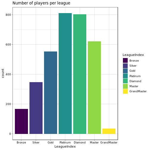
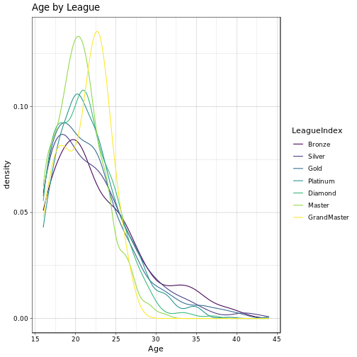
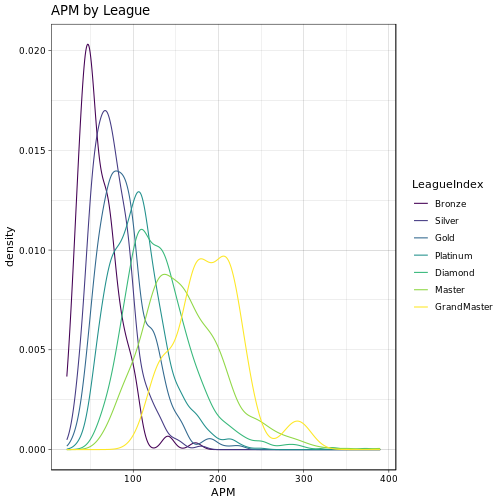
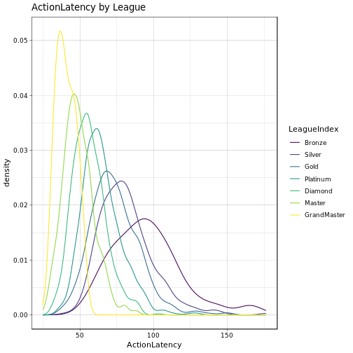
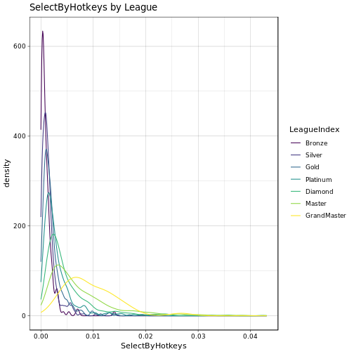
Above we can see some interesting stuff already. First think we notice is that most players reside somewhere in the ‘medium’ leagues’. It seems that it is relatively easy to progress to Platinum/Diamond, however, in order to advance to the Master or even GrandMaster league some serious skill is required. Age distribution is about the same over all the leasgues, no real surprises there, although in GrandMaster we seem to have a slightly younger population. High APM seem to be somewhat more common in the GrandMaster league than in the others. Now, ActionLatency and SelectByHotkeys look a bit more interesting. Apparently, most gamers in the GrandMaster league have a low latency and hence quick reaction to events (which would make sense). Similarly, Master and GrandMaster gamers seem to select there units using hotkeys more often than players in the other leagues. Overall, the mean of the distributions seems to wander from somewhere around 100 to maybe 30-40 as we go from Bronze to GrandMaster (ActionLatency) and likewise for the SelectByHotkeys variable. We can quickly check the means of the respective distributions:
## # A tibble: 7 x 3
##   LeagueIndex average_actionlatency average_selectbyhotkeys
##   <ord>                       <dbl>                   <dbl>
## 1 Bronze                       95.4                 0.00108
## 2 Silver                       81.3                 0.00154
## 3 Gold                         73.7                 0.00219
## 4 Platinum                     64.8                 0.00315
## 5 Diamond                      56.1                 0.00498
## 6 Master                       48.9                 0.00744
## 7 GrandMaster                  40.3                 0.00942
Indeed, the higher the league the lower the ActionLatency and the higher the SelectByHotkeys statistic.
Now let’s check on the TotalHours:
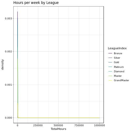
Zonk! Something’s wrong here! Seems that some few players have an extraordinary amount of played hours on their back, we should look at this in more detail!
Total hours played
Since we can’t really see anything in the plot, we check the table for some outliers. We get the table and sort it by TotalHours, decreasingly, and check the head:
| GameID | LeagueIndex | Age | TotalHours | APM | SelectByHotkeys | ActionLatency |
|---|---|---|---|---|---|---|
| 5140 | Diamond | 18 | 1000000 | 281.4246 | 0.0234282 | 36.1266 |
| 6518 | Master | 20 | 25000 | 247.0164 | 0.0157938 | 37.1837 |
| 2246 | Diamond | 22 | 20000 | 248.0490 | 0.0237032 | 45.3760 |
| 5610 | Platinum | 22 | 18000 | 152.2374 | 0.0119831 | 63.9811 |
| 6242 | Gold | 24 | 10260 | 76.5852 | 0.0007798 | 84.6340 |
| 72 | GrandMaster | 17 | 10000 | 212.6022 | 0.0090397 | 41.7671 |
Crazy! There is one player (age 18!) who has apparently a preposterous total of 1,000,000 played hours…
OK, let’s do the math, shall we? So 1,000,000 hours, that would be 41,666 days and about 114 years. Though we appreciate the effort, for the sake of our further analysis we should filter out unreasonable total hours in general.
NOTE: There’s a chance we interpreted the dataset wrong, since there is no real description available on Kaggle. Anyway, for now we just go with it.
We remove all players with TotalHours > 8.766 × 10⁴ (10 years) and check out the plots again:
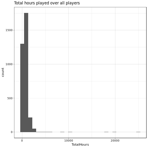
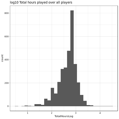
Ah, this looks much more like it! We can now see that we have only very few players who have about 20,000 TotalHours (2.2815423 years), still crazy! Let’s do the by-league plot once more (in log-space), and let’s again look at the means:
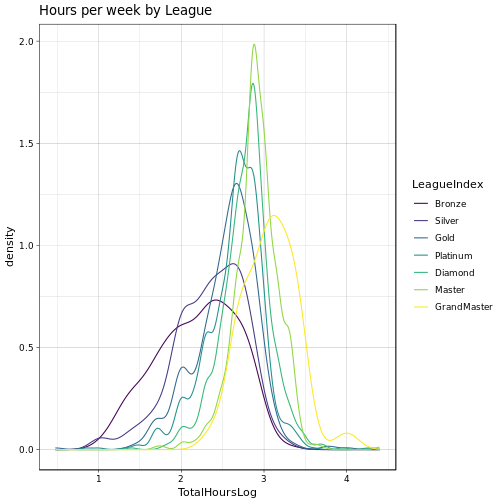
## # A tibble: 7 x 2
##   LeagueIndex `mean(TotalHours)`
##   <ord>                    <dbl>
## 1 Bronze                    264.
## 2 Silver                    331.
## 3 Gold                      494.
## 4 Platinum                  588.
## 5 Diamond                   782.
## 6 Master                    988.
## 7 GrandMaster              1581.
This satisfyingly feeds our expectations! On average, if you are placed in a higher league it seems that you did play the game for a longer period of time than your fellow ‘lower-leagures’!
LeagueIndex is indicative of APM, ActionLatency and TotalHours
Now we can check whether our favourite variables are indeed determined by the player’s current league placement.
First get an impression of whether a high amount of total hours played indicates a high APM or low ActionLatency. Again, we take the hours in log-space.
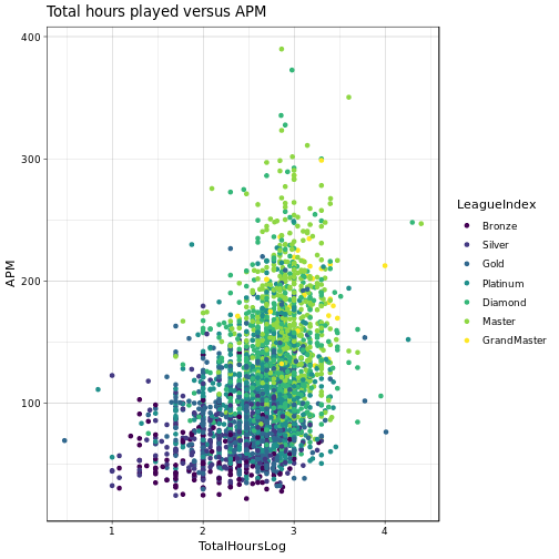
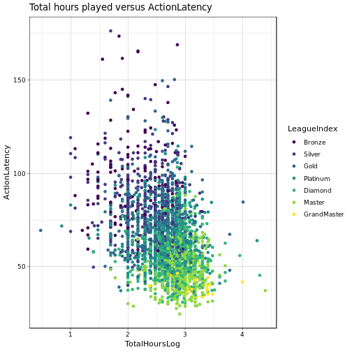
Ah, I like these plots, they allow us to extract some interesting information (and plainly look fancy!). We can see that in higher leagues in general the APM seem to be higher than in lower leagues, same for the TotalHours played. Similarly, ActionLatency is lower in higher leagues, also somewhat correlating with the TotalHours played.
Now we shall look at this information a bit differently, doing violin plots instead of these points:
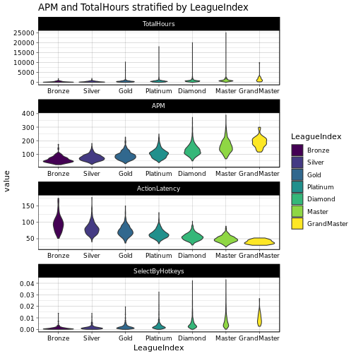
Here we can see quite clearly, that for each of the chosen variables, the LeagueIndex is indeed indicative of their values. We can further assess this using linear models. Now we train and report a linear model using LeagueIndex as the independent and our respective variables aus the dependent variables.
## [1] "Summary for APM model:"##
## Call:
## lm(formula = APM ~ LeagueIndex, data = sc_sub)
##
## Residuals:
## Min 1Q Median 3Q Max
## -93.310 -24.799 -3.938 19.251 241.251
##
## Coefficients:
## Estimate Std. Error t value Pr(>|t|)
## (Intercept) 115.6813 1.1068 104.514 < 2e-16 ***
## LeagueIndex.L 113.2522 4.0530 27.943 < 2e-16 ***
## LeagueIndex.Q 17.2389 3.8763 4.447 8.98e-06 ***
## LeagueIndex.C 1.9162 3.1178 0.615 0.539
## LeagueIndex^4 -2.4592 2.2813 -1.078 0.281
## LeagueIndex^5 0.1647 1.7361 0.095 0.924
## LeagueIndex^6 1.7045 1.4365 1.187 0.235
## ---
## Signif. codes: 0 '***' 0.001 '**' 0.01 '*' 0.05 '.' 0.1 ' ' 1
##
## Residual standard error: 37.22 on 3330 degrees of freedom
## Multiple R-squared: 0.4007, Adjusted R-squared: 0.3996
## F-statistic: 371.1 on 6 and 3330 DF, p-value: < 2.2e-16## [1] "Summary for TotalHours model:"##
## Call:
## lm(formula = TotalHours ~ LeagueIndex, data = sc_sub)
##
## Residuals:
## Min 1Q Median 3Q Max
## -1341.0 -288.4 -93.8 142.0 24011.6
##
## Coefficients:
## Estimate Std. Error t value Pr(>|t|)
## (Intercept) 718.36 24.47 29.355 < 2e-16 ***
## LeagueIndex.L 1049.30 89.61 11.710 < 2e-16 ***
## LeagueIndex.Q 332.53 85.70 3.880 0.000106 ***
## LeagueIndex.C 151.85 68.93 2.203 0.027673 *
## LeagueIndex^4 88.68 50.44 1.758 0.078808 .
## LeagueIndex^5 14.00 38.38 0.365 0.715322
## LeagueIndex^6 42.71 31.76 1.345 0.178768
## ---
## Signif. codes: 0 '***' 0.001 '**' 0.01 '*' 0.05 '.' 0.1 ' ' 1
##
## Residual standard error: 822.9 on 3330 degrees of freedom
## Multiple R-squared: 0.07834, Adjusted R-squared: 0.07668
## F-statistic: 47.18 on 6 and 3330 DF, p-value: < 2.2e-16## [1] "Summary for ActionLatency model:"##
## Call:
## lm(formula = ActionLatency ~ LeagueIndex, data = sc_sub)
##
## Residuals:
## Min 1Q Median 3Q Max
## -44.298 -9.118 -1.446 7.437 95.102
##
## Coefficients:
## Estimate Std. Error t value Pr(>|t|)
## (Intercept) 65.7943 0.4243 155.079 <2e-16 ***
## LeagueIndex.L -46.7588 1.5535 -30.098 <2e-16 ***
## LeagueIndex.Q 3.2909 1.4858 2.215 0.0268 *
## LeagueIndex.C -2.1009 1.1951 -1.758 0.0788 .
## LeagueIndex^4 1.1509 0.8744 1.316 0.1882
## LeagueIndex^5 -1.4994 0.6655 -2.253 0.0243 *
## LeagueIndex^6 0.1835 0.5506 0.333 0.7389
## ---
## Signif. codes: 0 '***' 0.001 '**' 0.01 '*' 0.05 '.' 0.1 ' ' 1
##
## Residual standard error: 14.27 on 3330 degrees of freedom
## Multiple R-squared: 0.4393, Adjusted R-squared: 0.4383
## F-statistic: 434.8 on 6 and 3330 DF, p-value: < 2.2e-16## [1] "Summary for SelectByHotkeys model:"##
## Call:
## lm(formula = SelectByHotkeys ~ LeagueIndex, data = sc_sub)
##
## Residuals:
## Min 1Q Median 3Q Max
## -0.007315 -0.002049 -0.000855 0.000707 0.037302
##
## Coefficients:
## Estimate Std. Error t value Pr(>|t|)
## (Intercept) 4.252e-03 1.253e-04 33.929 < 2e-16 ***
## LeagueIndex.L 7.480e-03 4.589e-04 16.300 < 2e-16 ***
## LeagueIndex.Q 2.014e-03 4.389e-04 4.589 4.61e-06 ***
## LeagueIndex.C -1.358e-04 3.530e-04 -0.385 0.700
## LeagueIndex^4 -4.239e-04 2.583e-04 -1.641 0.101
## LeagueIndex^5 -1.552e-04 1.966e-04 -0.789 0.430
## LeagueIndex^6 2.754e-05 1.627e-04 0.169 0.866
## ---
## Signif. codes: 0 '***' 0.001 '**' 0.01 '*' 0.05 '.' 0.1 ' ' 1
##
## Residual standard error: 0.004214 on 3330 degrees of freedom
## Multiple R-squared: 0.2026, Adjusted R-squared: 0.2012
## F-statistic: 141 on 6 and 3330 DF, p-value: < 2.2e-16As you can see, again we observe that we have a linear dependence between all our variabels and the LeagueIndex. We probably should explore this a bit more, but for now let’s go on with predicting league placement!
Predicting league placement
Great! Some machine learning for predicting league placement, eh? (don’t worry, this will be very high-level and we don’t go into much detail for now). We build a random forest model (i.e. an ensembl of decision trees, wiki link) using the randomForest package by Breiman and Cutler available on CRAN. In the model we use all our variables as inputs and try to model the LeagueIndex using default parameters except for the number of trees which we set to 10,000.
NOTE: Again, this is not a very sophisticated approach as we do it here, we just wanna see how good we can get by blindly applying this model. We’ll probably return to this at a later point.
## Error in library(randomForest): there is no package called 'randomForest'## Error in randomForest(LeagueIndex ~ ., data = data, ntree = 10000): could not find function "randomForest"## Error in print(model): object 'model' not foundPerformance
Wonderful, we got some results! Hmmm, but what do we see here? Apparently, unfortunately we were not able to do a satisfying job (out-of-bag error rate (OOB) around 64%!). Well, let’s move on for now.
Mock predictions
Looking at the confusion matrix, however, we seem to be fairly ‘close’ with most predictions (if we assume that e.g. Silver league is similar to Bronze and Gold, etc.). Since this analysis is just for fun, let’s define new ‘mock’ leagues, deviding players into ‘good’ and ‘bad’ ones. Maybe we can do better on these two classes?
## Error in randomForest(LeagueIndex ~ ., data = sc_mock, ntree = 10000): could not find function "randomForest"## Error in print(model_mock): object 'model_mock' not foundAs we can see the OOB is a lot better at about 22%, it’s something!
Feature importance
Finally, let’s quickly check on the feature importance for the mock predictions.
## Error in eval(expr, envir, enclos): object 'model_mock' not foundThe MeanDecreaseGini is highest for the ActionLatency, suggesting that this variable is the most important one for predicting ‘bad’ and ‘good’ players in our mock prediction experiment (the higher the index in general, the ‘more important’ the respective variable).
Conclusion
We looked at some of the more intuitive variables accessible in the SkillCraft dataset and got a nice feel of the data using rather straight forward ggplot functionality.
Overall, we were able to see that the league placement already gives a hint on the average APM, ActionLatency and TotalHours played for each player.
We finished with some experimental machine learning on these data, simply applying randomForests on the three variables to predict the LeagueIndex. Whereas for the multi-class case this didn’t work well, for a mock prediction experiement were we replaced the LeagueIndex naivly with a two-class label we obtained ‘ok’ results.
This could be followed up by a more sophisticated approach, using more variables, doing some serious variable selection and normalization prior to applying any model and finally evaluating the results using e.g. the AUC or F1 measure.
But for now we are happy with what we have done and can go on to the next task!
Until then, farewell!
-or-
Khas il’adare - for anyone ‘speaking’ Khalani
Session Info
## R version 3.4.4 (2018-03-15)
## Platform: x86_64-pc-linux-gnu (64-bit)
## Running under: Ubuntu 18.04.1 LTS
##
## Matrix products: default
## BLAS: /usr/lib/x86_64-linux-gnu/blas/libblas.so.3.7.1
## LAPACK: /usr/lib/x86_64-linux-gnu/lapack/liblapack.so.3.7.1
##
## locale:
##  [1] LC_CTYPE=C.UTF-8       LC_NUMERIC=C           LC_TIME=C.UTF-8
##  [4] LC_COLLATE=C.UTF-8     LC_MONETARY=C.UTF-8    LC_MESSAGES=C.UTF-8
##  [7] LC_PAPER=C.UTF-8       LC_NAME=C              LC_ADDRESS=C
## [10] LC_TELEPHONE=C         LC_MEASUREMENT=C.UTF-8 LC_IDENTIFICATION=C
##
## attached base packages:
## [1] stats     graphics  grDevices utils     datasets  base
##
## other attached packages:
##  [1] bindrcpp_0.2.2  reshape2_1.4.3  forcats_0.3.0   stringr_1.3.1
##  [5] dplyr_0.7.8     purrr_0.3.0     readr_1.3.1     tidyr_0.8.2
##  [9] tibble_2.0.1    ggplot2_3.1.0   tidyverse_1.2.1 knitr_1.21
##
## loaded via a namespace (and not attached):
##  [1] Rcpp_1.0.0        highr_0.7         cellranger_1.1.0
##  [4] pillar_1.3.1      compiler_3.4.4    plyr_1.8.4
##  [7] bindr_0.1.1       methods_3.4.4     tools_3.4.4
## [10] digest_0.6.18     viridisLite_0.3.0 lubridate_1.7.4
## [13] jsonlite_1.6      evaluate_0.12     nlme_3.1-131
## [16] gtable_0.2.0      lattice_0.20-35   pkgconfig_2.0.2
## [19] rlang_0.3.1       cli_1.0.1         rstudioapi_0.9.0
## [22] haven_2.0.0       xfun_0.4          withr_2.1.2
## [25] xml2_1.2.0        httr_1.4.0        hms_0.4.2
## [28] generics_0.0.2    grid_3.4.4        tidyselect_0.2.5
## [31] glue_1.3.0        R6_2.3.0          fansi_0.4.0
## [34] readxl_1.2.0      modelr_0.1.2      magrittr_1.5
## [37] backports_1.1.3   scales_1.0.0      rvest_0.3.2
## [40] assertthat_0.2.0  colorspace_1.4-0  labeling_0.3
## [43] utf8_1.1.4        stringi_1.2.4     lazyeval_0.2.1
## [46] munsell_0.5.0     broom_0.5.1       crayon_1.3.4
Comments