Analysis of a thyroid gene expression dataset
Inroduction
This is an exploratory analysis of the downloaded and processed ARCHS4 gene expression data for a thyroid tissue specification. Here we want to get an idea of how uniform these data are and whether additional (manual) curation would be necessary prior to any downstream analysis.
NOTE: All data were obtained from ARCHS4 using the ARCHS4 data loader (under development)
Gene expression data
The central dogma of biology states that genes on the DNA of a cell are transcribed into RNAs which are in turn further processed and translated into proteins. Modern experimental technologies such as next-generation sequencing enable researchers to obtain a complete read-out of RNA molecules present in a specific biosample at the time of measurement. These read-outs can be quantified on a per gene (or per transcript) basis to obtain gene expression data: A quantitative recording of the amount of RNA molecules per gene present in individual biosamples (ofter a mixture of cells of a specific tissue, such as the thyroid in our case). Using these estimates, scientist seek to answer pressing biomedical questions such as the identification of the molecular mechanisms behind cancer or other diseases.
ARCHS4
Typically, a gene expression dataset is comprised of relatively few samples (ten to several hundred) as compared to the number of quantified genes (tens of thousands) making statistical analysis challenging. Gene expression data can be gathered using diverse experimental protocols and hence data obtained from different laboratories can usually not be analyzed ‘as is’ in any meta study seeking to harvest a larger sample size which is often limited for individual studies. ARCHS4 is a project which seeks to unite gene expression data form diverse laboratories and provide easy access to a homogeneously processed data matrix, containing hundreds to thousands of individual samples ready for a joint analysis. This increased sample size could potentially yield a higher statistical power to discover e.g. functional molecular pathways.
NOTE: A detailed overview on ARCHS4 can be found on the ARCHS4 homepage or in the respective publication.
t-SNE
To visualize and get an impression of our gene expression data we utilize the t-SNE algorithm. Briefly, t-SNE is a dimension reduction technique (think of e.g. PCA or your other favourite dimension reduction method) which enables us to obtain a low dimensional (say, 2-3 dimensions) representation of a high dimensional (e.g. several thousands, as with gene expression data). We can use this low dimensional representation to nicely display our data on a simple 2-dimensional space, such as a regular x-y plot. In this representation, very similar samples will be close to each other and hence form clusters. These we can then interpret by e.g. coloring the individual points with specific sample annotations.
Let’s start!
Exploration
In this analysis we will have have a look at the raw gene counts as well as the normalized expression matrix as provided by the ARCHS4 loader.
NOTE: I will not go into more details regarding ‘gene counts’ or ‘normalization’. Both are quantitative values of the amount of RNA present in a cell per specific gene, the former being the ‘direct readouts’ from the sequencing machine (after some initial processing) and the latter is adjusted for sources of unwanted variation which could have influenced our readouts, such as different length of genes, differences in sample preparation during the experiment etc.
After loading the data, we see that we have a total of 35238 genes measured in 143 samples (same for both raw and normalized data). Below is a sample of the raw data matrix:
| gene_name | GSM742951 | GSM913883 | GSM913881 | GSM1185644 | GSM913884 | GSM1185638 | GSM913876 | GSM913888 | GSM1185640 |
|---|---|---|---|---|---|---|---|---|---|
| A1BG | 0 | 196 | 268 | 189 | 73 | 263 | 148 | 114 | 373 |
| A1CF | 0 | 2 | 0 | 2 | 0 | 7 | 1 | 2 | 11 |
| A2M | 545 | 725 | 751 | 11707 | 243 | 13394 | 308 | 1040 | 20788 |
| A2ML1 | 0 | 40 | 42 | 8 | 7 | 29 | 5 | 7 | 47 |
| A2MP1 | 0 | 0 | 2 | 5 | 1 | 19 | 0 | 3 | 42 |
We can already see that there are quite some differences in the number of counts per gene and sample (e.g. 0 vs 13394). Let’s have a brief look a the distribution of counts.
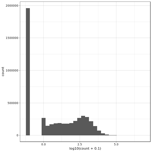
Alright, we see that there are a lot of zeros involved (notice that we used log10 transformation and added pseudo-count to get rid of -Inf values). Actually, this seems like rather more zeros than we would maybe expect. Let’s check also the proportion of zeros per gene and per sample over all genes and samples, respectively.
##  GSM742951  GSM913883  GSM913881 GSM1185644  GSM913884 GSM1185638
##  0.8515239  0.4226120  0.4138714  0.3695442  0.4965662  0.3180090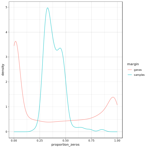
The above plot shows the density of the proportion of zero valued entries for each of the genes (red) and each of the samples (blue). We can observe that we have several genes which seem to have virtually no counts at all. We will filter these out prior to processing in addition to all genes which do not show any variation across the samples. Furthermore, we observe that most of the samples have a moderate amount of non-expressed genes which feeds our expectations.
Filtering out lowly expressed and non varying genes leaves us with 33249 genes.
In addition to the expression data, the ARCHS4 loader provides us with a design table containing the following column names(already somewhat adjusted for better readability):
## [1] "sample"          "tissue"          "series"          "organism"
## [5] "molecule"        "characteristics" "description"     "instrument"
Before looking in detail at the expression data, we first have a look at the individual columns of the design table in order to better get to know our data. Below we show for each column of the design matrix the unique values contained therein. This is a bit messy, but for now we accept this:
## [[1]]
## # A tibble: 15 x 1
##    tissue
##    <chr>
##  1 thyroid
##  2 parathyroid adenoma
##  3 thyroid tissue
##  4 primary thyroid cell line
##  5 thyroid cancer cells
##  6 non-medullary thyroid carcinoma cell line
##  7 thyroid gland tissue female fetal (40 weeks)
##  8 thyroid gland tissue female fetal (37 weeks)
##  9 thyroid gland tissue male adult (54 years)
## 10 thyroid gland tissue male adult (37 years)
## 11 thyroid gland tissue female adult (51 year)
## 12 thyroid gland tissue female adult (53 years)
## 13 papillary thyroid cancer invasive region
## 14 papillary thyroid cancer central region
## 15 papillary thyroid
##
## [[2]]
## # A tibble: 2 x 1
##   molecule
##   <chr>
## 1 polyA RNA
## 2 total RNA
##
## [[3]]
## # A tibble: 75 x 1
##    characteristics
##    <chr>
##  1 library type: single-endXx-xXread length: 50
##  2 patient: 2Xx-xXtissue: Parathyroid tumorXx-xXagent: OHTXx-xXtime: 24h
##  3 patient: 2Xx-xXtissue: Parathyroid tumorXx-xXagent: DPNXx-xXtime: 24h
##  4 disease state: TumorXx-xXtissue: thyroid
##  5 patient: 2Xx-xXtissue: Parathyroid tumorXx-xXagent: OHTXx-xXtime: 48h
##  6 disease state: NormalXx-xXtissue: thyroid
##  7 patient: 1Xx-xXtissue: Parathyroid tumorXx-xXagent: DPNXx-xXtime: 48h
##  8 patient: 3Xx-xXtissue: Parathyroid tumorXx-xXagent: DPNXx-xXtime: 48h
##  9 patient: 1Xx-xXtissue: Parathyroid tumorXx-xXagent: ControlXx-xXtime: 2…
## 10 patient: 2Xx-xXtissue: Parathyroid tumorXx-xXagent: ControlXx-xXtime: 4…
## # … with 65 more rows
##
## [[4]]
## # A tibble: 4 x 1
##   instrument
##   <chr>
## 1 Illumina HiSeq 2000
## 2 Illumina HiSeq 2500
## 3 Illumina NextSeq 500
## 4 Illumina HiSeq 4000
We can see that the ‘tissue’ meta data (‘source’ in the original ARCHS4 definition) contains several different but Thyroid related tissues. In addition, experiments differ by the type of extracted molecules (polyA RNA, i.e. processed mRNA and total RNA, i.e. all RNA found in the cell) and we can see that different instruments (i.e. sequencing machines) have been used to create sequencing information.
For us, the tissue information is most interesting. Let’s see what we get in terms of sample counts if we group by the individual ‘tissues’:
## # A tibble: 15 x 2
##    tissue                                       count
##    <chr>                                        <int>
##  1 thyroid tissue                                  35
##  2 thyroid                                         30
##  3 non-medullary thyroid carcinoma cell line       27
##  4 parathyroid adenoma                             23
##  5 thyroid cancer cells                             8
##  6 papillary thyroid cancer central region          3
##  7 papillary thyroid cancer invasive region         3
##  8 primary thyroid cell line                        2
##  9 thyroid gland tissue female adult (53 years)     2
## 10 thyroid gland tissue female fetal (37 weeks)     2
## 11 thyroid gland tissue female fetal (40 weeks)     2
## 12 thyroid gland tissue male adult (37 years)       2
## 13 thyroid gland tissue male adult (54 years)       2
## 14 papillary thyroid                                1
## 15 thyroid gland tissue female adult (51 year)      1
As we can see there is some diversity in this column. We can also see, however, that we can probably combine some of these annotations since they seem very similar (look e.g. at the ‘thyroid tissue’ and ‘thyroid’ annotation). If we’d want to extract a dataset as homogeneous as possible from these data we could consider doing this in a more elaborate way, for now we just create a new column in which we define two new tissue groups: thyroid cancer and thyroid.
| tissue_group | count |
|---|---|
| thyroid | 79 |
| thyroid (cancerous) | 64 |
Raw and batch normalized gene expression
Ok, now let’s have a closer look at the actual gene expression data. We will have a look at the histogram of all expression values and a heatmap of the top 1% most variable genes. We will do this both for the normalized data as well as the raw gene expression counts for comparison, note that we already filtered out lowly expressed and non-varying genes:
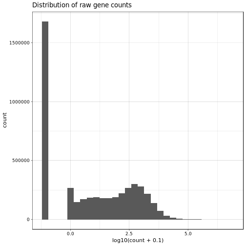
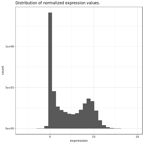
Nothing very unexpected about these two histograms. In general we can observe a slight enrichment of lowly and highly expressed genes and relatively less moderately expressed genes.
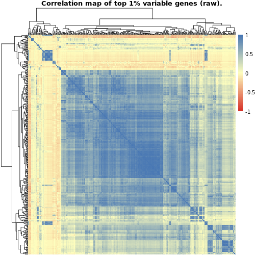
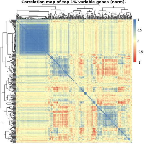
The first plot, showing the correlations between the raw gene counts, indicates quite a lot of strongly positive correlated genes whereas the second plot showing the normalized data provides a more balanced picture of positively and negatively correlated genes. In both cases, though, we seem to have a certain cluster of genes which evidence a strong positive correlation. These could indicate genes playing important regulatory roles in thyroid (maybe hormone binding related?) which they regulate in a coordinated fashion.
NOTE: We could check this assumption by performing e.g. gene ontology enrichment using this identified set of genes and evaluating the significant terms which would pop up in the analysis
t-SNE
Now let’s do some of these t-SNE plots to see whether we can observe any specific clusters emerging. Again we will look at two distinct plots: One for the raw expression data and one for the normalized data.
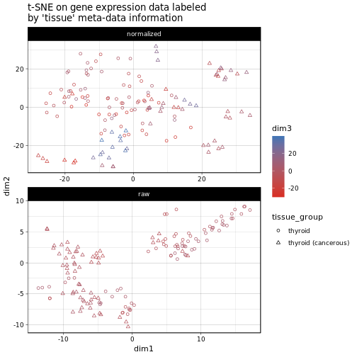
Here each point is a sample and we plotted the first two t-SNE dimensions on the x and y axis and indicate the third dimension as the color of the respective points. The shape of the individual points reflects the sample’s tissue group, i.e. either ‘thyroid’ or ‘thyroid (cancerous)’ as per our definition. for the normalized data we can’t really see any clusters emerging, with the small exception of a several cancerous samples on the border areas of the plot. In the raw count case we see a slight separation of two clusers which match relatively well with our tissue group definitions (though by no means perfectly). This indicates that, using the batch normalized expression data we obtain a more or less heterogeneous set of samples, however, the cancerous samples should still be treated with care or even removed prior to any downstream analysis (seeing that gene expression is often largely disrupted in cancer this also makes sense from a biologcial perspective).
Finally, we see whether the used instrument of the sequencing experiment is captued within the first two dimensions of the t-SNE (we use the color to indicate the instrument now, since here we have more than 2 groups and this is easier to get a hold of):
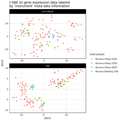
In this case we cannot really see any clear clusters emerging, with the possible exception of the Illumina HiSeq 4000 in the center of the raw count plot. Anyway, any differences in the data due to the used instrument seem to be successfully removed after batch normalization.
Conclusion
In this analysis we took a look at the thyroid related gene expression data available in the ARCHS4 database. In general, we could see that the data are rather diverse in terms of tissue annotation, but can to some extend be merged together to obtain a more homogeneous annotation. The t-SNE plots indicate that the cancerous samples, as expected, are still quite different to the ‘healthy’ samples in the data. So in any downstream analysis, one would want to consider removing these samples in order to obtain a well defined, homogeneous dataset from which further conclusions can be drawn. Alternatively, one could aim at performing a differential expression analysis to identify genes which are either up- or downregulated in the cancer tissue, hence identifying genes crucial to understanding cancer related biological mechanisms.
That’s it for today, hope you enjoyed the analysis and I’m lookgin forward to any feedback and suggestions for this post.
Until then, farewell!
Session Info
## R version 3.4.4 (2018-03-15)
## Platform: x86_64-pc-linux-gnu (64-bit)
## Running under: Ubuntu 18.04.1 LTS
##
## Matrix products: default
## BLAS: /usr/lib/x86_64-linux-gnu/blas/libblas.so.3.7.1
## LAPACK: /usr/lib/x86_64-linux-gnu/lapack/liblapack.so.3.7.1
##
## locale:
##  [1] LC_CTYPE=C.UTF-8       LC_NUMERIC=C           LC_TIME=C.UTF-8
##  [4] LC_COLLATE=C.UTF-8     LC_MONETARY=C.UTF-8    LC_MESSAGES=C.UTF-8
##  [7] LC_PAPER=C.UTF-8       LC_NAME=C              LC_ADDRESS=C
## [10] LC_TELEPHONE=C         LC_MEASUREMENT=C.UTF-8 LC_IDENTIFICATION=C
##
## attached base packages:
## [1] stats     graphics  grDevices utils     datasets  base
##
## other attached packages:
##  [1] RColorBrewer_1.1-2 Rtsne_0.15         pheatmap_1.0.12
##  [4] bindrcpp_0.2.2     reshape2_1.4.3     forcats_0.3.0
##  [7] stringr_1.3.1      dplyr_0.7.8        purrr_0.3.0
## [10] readr_1.3.1        tidyr_0.8.2        tibble_2.0.1
## [13] ggplot2_3.1.0      tidyverse_1.2.1    knitr_1.21
##
## loaded via a namespace (and not attached):
##  [1] tidyselect_0.2.5  xfun_0.4          haven_2.0.0
##  [4] lattice_0.20-35   colorspace_1.4-0  generics_0.0.2
##  [7] viridisLite_0.3.0 utf8_1.1.4        rlang_0.3.1
## [10] pillar_1.3.1      glue_1.3.0        withr_2.1.2
## [13] modelr_0.1.2      readxl_1.2.0      bindr_0.1.1
## [16] plyr_1.8.4        munsell_0.5.0     gtable_0.2.0
## [19] cellranger_1.1.0  rvest_0.3.2       codetools_0.2-15
## [22] evaluate_0.12     labeling_0.3      fansi_0.4.0
## [25] highr_0.7         broom_0.5.1       methods_3.4.4
## [28] Rcpp_1.0.0        scales_1.0.0      backports_1.1.3
## [31] jsonlite_1.6      hms_0.4.2         digest_0.6.18
## [34] stringi_1.2.4     grid_3.4.4        cli_1.0.1
## [37] tools_3.4.4       magrittr_1.5      lazyeval_0.2.1
## [40] crayon_1.3.4      pkgconfig_2.0.2   xml2_1.2.0
## [43] lubridate_1.7.4   assertthat_0.2.0  httr_1.4.0
## [46] rstudioapi_0.9.0  R6_2.3.0          nlme_3.1-131
## [49] compiler_3.4.4
Comments